darius is studying the relationship between mathematics and art. he asks friends to each draw a “typical”…
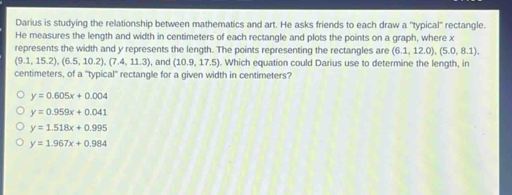
darius is studying the relationship between mathematics and art. he asks friends to each draw a “typical” rectangle. he measures the length and width in centimeters of each rectangle and plots the points on a graph, where x represents the width and y represents the length. the points representing the rectangles are (6.1, 12.0), (5.0, 8.1), (9.1, 15.2), (6.5, 10.2), (7.4, 11.3), and (10.9, 17.5). which equation could darius use to determine the length, in centimeters, of a “typical” rectangle for a given width in centimeters?\no y = 0.605x + 0.004\no y = 0.959x + 0.041\no y = 1.518x + 0.995\no y = 1.967x + 0.984
Answer
Explanation:
Step1: Recall linear - regression concept
We want to find the line of best - fit for the data points ((x,y)) which has the form (y = mx + b), where (m) is the slope and (b) is the y - intercept. One way is to use a calculator with linear - regression capabilities. Another way is to check each equation by substituting some of the (x) values from the data points and seeing which equation gives (y) values closest to the actual (y) values in the data. Let's take the first data point ((x = 6.1,y = 12.0)) and substitute into each equation:
For (y=0.605x + 0.004):
Substitute (x = 6.1) into the equation: (y=0.605\times6.1+0.004=0.605\times6.1 + 0.004=3.6905+0.004 = 3.6945)
For (y = 0.959x+0.041):
Substitute (x = 6.1) into the equation: (y=0.959\times6.1 + 0.041=5.8499+0.041=5.8909)
For (y=1.518x + 0.995):
Substitute (x = 6.1) into the equation: (y=1.518\times6.1+0.995=9.2598 + 0.995=10.2548)
For (y=1.967x+0.984):
Substitute (x = 6.1) into the equation: (y=1.967\times6.1+0.984=12.0987+0.984 = 13.0827)
Let's take another data point ((x = 5.0,y = 8.1))
For (y=0.605x + 0.004):
(y=0.605\times5.0+0.004=3.025 + 0.004=3.029)
For (y = 0.959x+0.041):
(y=0.959\times5.0+0.041=4.795+0.041 = 4.836)
For (y=1.518x + 0.995):
(y=1.518\times5.0+0.995=7.59+0.995 = 8.585)
For (y=1.967x+0.984):
(y=1.967\times5.0+0.984=9.835+0.984=10.819)
By comparing the calculated (y) values with the actual (y) values of the data points, we can see that the equation (y = 1.518x+0.995) gives values that are relatively closer to the actual (y) values of the data points.
Answer:
(y = 1.518x+0.995)